From Binance Scripts to a Reusable Python Data Package

HdWCryptoData combines Binance Vision archives and recent REST API candles into analysis-ready pandas DataFrames—installable directly from PyPI.

HdWCryptoData combines Binance Vision archives and recent REST API candles into analysis-ready pandas DataFrames—installable directly from PyPI.

For several years, I have used a collection of Python scripts to download historical cryptocurrency data from Binance, combine it with recent market data and then prepare the resulting time series for analysis.

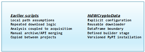
The scripts worked, but they retained the usual limitations of project-specific utilities: local folder assumptions, repeating setup and configuration tuning, tight coupling to analytical code and the absence of a clean reusable interface for other applications.

Now that has changed. To remove that recurring friction, in my project HdWCryptoData over the past few weeks I have intensively been refactoring and systematizing the diverse versions of the scripts into a coherent, lightweight, standalone data-retrieval package.

The result is hdw_crypto_data, a small Python package now available from PyPI and documented on GitHub. You can download and install it with: python -m pip install hdw-crypto-data.

This package turns the original intended workflow into a reusable data pipeline. It downloads historical candlestick data from Binance Vision, supplements those archives with recent candles from the Binance REST API and then merges and loads the result as a cleaned, timezone-aware pandas DataFrame.

This first release has reached version 0.1.0. It is still a young package, but it has already replaced the separate Binance data scripts in my own workflows.

Why two Binance clients are needed

Binance Vision is a well-known source for historical market data. It provides downloadable archives containing monthly and daily kline (candlestick) files. Each kline represents price action over a specific time interval (mostly 1 hour, but varies from 1 second to 1 month), the data for each candlestick consisting of four primary price points: Open, High, Low and Close and volume and number of trades added. These archives are suited to (and intended for) reconstructing a long time series without issuing thousands of individual REST requests.

An archive however, is not the same thing as a continuously current market feed. The newest periods may not yet be present in a monthly or daily archive. For an analysis that should extend into the present, historical files alone are not enough.

My HdWCryptoData project deliberately treats the two primary sources as complementary. Binance Vision supplies the historical monthly and daily kline archives. The Binance REST API supplies the most recent hourly candles. The dataset-builder merges the historical and recent data into one ordered dataset. The dataset-loader converts the result into a pandas DataFrame suitable for further processing.

This distinction is also why the original downloader class was renamed from BinanceDataDumper to BinanceVisionDumper. This downloader has a specific responsibility, retrieving the archive side of the pipeline. Creating the complete dataset requires both Binance Vision and the REST API.

The archive and API sources can overlap; the builder orders observations and removes duplicate periods before loading.

From a collection of scripts to a defined pipeline

The new hdw-crypto-data package separates the process into three main responsibilities.

1. Download historical data

BinanceVisionDumper retrieves the requested Binance Vision kline archives. It supports monthly files for older periods and daily files for the current month, following the Binance Vision directory structure. Before actually starting a download, it also checks which part of the requested history is already present locally. After completing a calendar month it removes the superfluous daily archives, thus keeping the local storage in sync with Binance Vision.  

The downloader now does (a lot) more than issue a request and unzip whatever comes back. For security we make use of a verified TLS connection, retry handling and Binance-specific URL validation. Since Binance publishes a checksum per archive, we also check the downloaded ZIP against this checksum before extraction.

Missing files, invalid archives and checksum mismatches are reported explicitly (rather than silently producing a possibly incomplete dataset).

from datetime import date
from hdw_crypto_data import BinanceVisionDumper

dumper = BinanceVisionDumper(
    path_dir_where_to_dump=r"D:\CryptoData\spot",
    asset_class="spot",
    data_type="klines",
    data_frequency="1h",
)

dumper.dump_data(
    tickers=["BTCUSDT", "ETHUSDT", "SOLUSDT"],
    date_start=date(2021, 1, 1),
    date_end=date.today(),
)

from datetime import date
from hdw_crypto_data import BinanceVisionDumper

dumper = BinanceVisionDumper(
    path_dir_where_to_dump=r"D:\CryptoData\spot",
    asset_class="spot",
    data_type="klines",
    data_frequency="1h",
)

dumper.dump_data(
    tickers=["BTCUSDT", "ETHUSDT", "SOLUSDT"],
    date_start=date(2021, 1, 1),
    date_end=date.today(),
)

The market pairs are explicit. In the trading pair BTCUSDT, Bitcoin is the base currency. It is collected against USDT, the quote currency, that is the unit of measurement used to price the base currency.

Note. Market data on Binance Vision does not require an account or private API key.

2. Build the total dataset

Once the historical archives are available locally, TotalDatasetBuilder collects the recent candles from the Binance REST API and merges them with the locally stored monthly and daily files. The builder produces one ordered, deduplicated time series spanning the available historical archives and recent API observations, while making missing periods detectable.

from hdw_crypto_data import TotalDatasetBuilder

builder = TotalDatasetBuilder(
    asset="BTC",
    settings="settings.json",
    force_merge=False,
)

result = builder.build()
print(result.filepath)
print(f"{result.rows:,} rows")

from hdw_crypto_data import TotalDatasetBuilder

builder = TotalDatasetBuilder(
    asset="BTC",
    settings="settings.json",
    force_merge=False,
)

result = builder.build()
print(result.filepath)
print(f"{result.rows:,} rows")

The generated file follows a simple naming convention, such as: BTCUSDT-total.csv.

During the merge, the builder brings the different file periods together, orders the rows and removes overlap between archive data and recent API data. This produces a single time series instead of leaving every analysis script to rediscover how monthly, daily and live files relate to one another.

A minimal `settings.json` can identify the local Binance data tree, preferred time zone and quote currency:

{
  "full_spot": "D:\\CryptoData\\spot",
  "preferred_time_zone": "Europe/Amsterdam",
  "quote_currency": "USDT"
}

{
  "full_spot": "D:\\CryptoData\\spot",
  "preferred_time_zone": "Europe/Amsterdam",
  "quote_currency": "USDT"
}

3. Load an analysis-ready DataFrame

TotalDatasetLoader reads the total CSV, normalizes timestamps, converts the index to the preferred time zone and returns a pandas DataFrame.

from hdw_crypto_data import TotalDatasetLoader

loader = TotalDatasetLoader("BTC", "settings.json")
df = loader.load_total_dataframe(
    mode="ta",				# intended use is technical analysis
    preferred_tz="Europe/Amsterdam",
)
print(df.tail())
print(df.index.min(), "to", df.index.max())

from hdw_crypto_data import TotalDatasetLoader

loader = TotalDatasetLoader("BTC", "settings.json")
df = loader.load_total_dataframe(
    mode="ta",				# intended use is technical analysis
    preferred_tz="Europe/Amsterdam",
)
print(df.tail())
print(df.index.min(), "to", df.index.max())

In technical-analysis mode, the result contains the familiar OHLC fields together with useful trading activity columns, indexed by localized datetimes.

The important outcome is not the CSV itself: it is the DataFrame boundary. Once the data is represented consistently as a DataFrame, downstream code no longer needs to know which rows came from a monthly ZIP, a daily file or the REST API.

That makes the package useful as infrastructure rather than as a single-purpose analysis script.

A PyQt Showcase using the Complete Workflow

The GitHub repository includes a PyQt showcase application that exercises the pipeline visually.

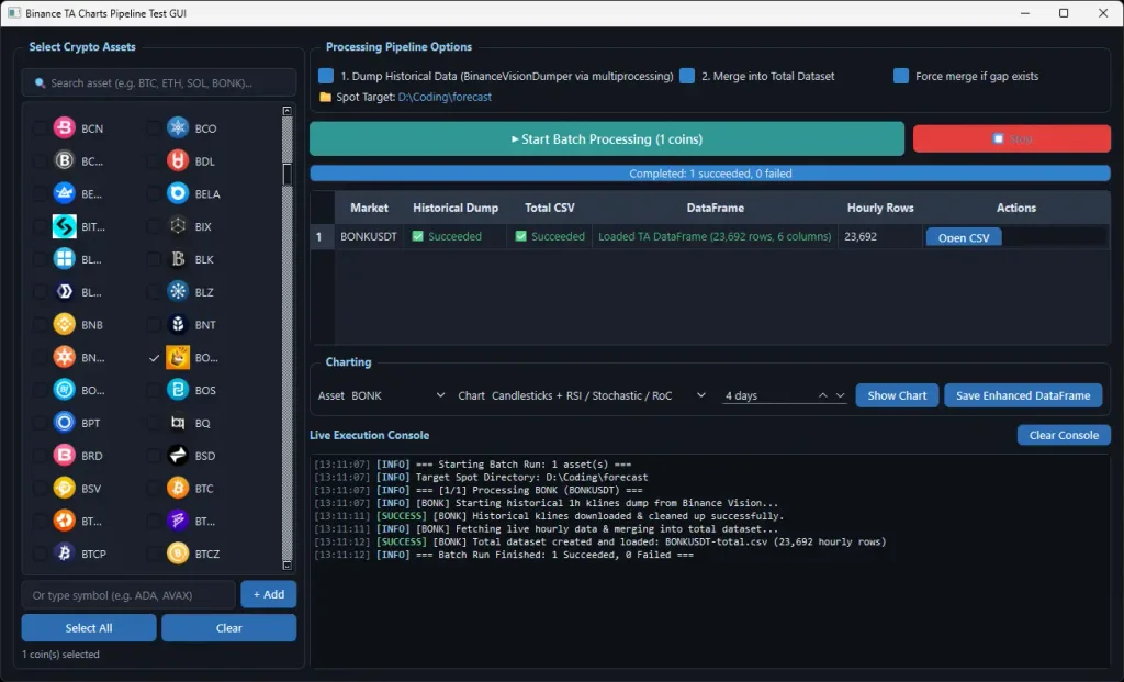
The application presents a searchable collection of crypto assets with recognizable coin icons. Multiple assets can be selected, after which the application can run the download, build and load stages without requiring the user to assemble each call manually. Progress and results are displayed in the interface, making it easier to follow what the package is doing and to test different markets.

The visual interface layer is intentionally kept outside the lightweight core package. Users who only want DataFrames do not need to import PyQt, Plotly and a collection of technical-analysis dependencies. A data package should not force a graphical application—or its dependency tree—onto every notebook, server process or machine-learning environment that uses it.

The showcase application and analysis extras can be downloaded and installed separately.

Demonstrating the Technical-Analysis Use-case

The showcase includes a series of technical-analysis charts built with the optional TACharts helper. It turns the loaded DataFrame into an interactive Plotly visualization with price data and technical indicators.

This makes technical analysis a useful demonstration because it exercises the full path just discussed. Retrieve a long historical record, extend it with recent candles, normalize the time axis and inspect continuity and missing observations. Then use the resulting DataFrame to calculate the indicators and display the result interactively.

It also makes an important architectural point visible: the charting code just consumes the DataFrame. It does not need to know about the downloading or merging logic.

After retrieving the data, you can interactively experiment with the visualizations in this showcase application, by varying the relevant range of the time series.

Overview of Available Charts

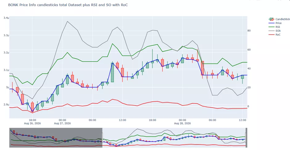
One consumer of the resulting DataFrame: an interactive technical-analysis view. The charting layer does not need to know how the underlying observations were downloaded or merged.

A convenient feature is that Plotly plots each chart separately or in a tab in the default browser. This allows you to have multiple charts open simultaneously to browse and compare them.

Note. The indicators and signals in the showcase charts are exploratory. Their purpose is to demonstrate how the same consistently indexed DataFrame can support varied analytical views.

Interpolation

The loader can also detect gaps and, when requested, fill missing hourly observations. That behaviour should be selected consciously. Interpolated values can be practical for charting or particular numerical methods, but they are synthetic observations and may be inappropriate as training targets or evidence of actual traded prices. For serious analysis, retaining a record of missing timestamps and documenting the chosen cleaning policy is essential.

The DataFrame is the real product boundary

Technical analysis, although a broad and varied field of application, is only one possible consumer of DataFrames.

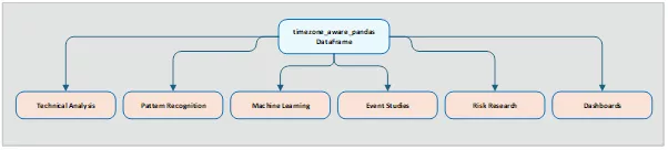
One DataFrame, many applications.

Pattern Recognition & Machine Learning

The same consistently indexed time series could also support pattern recognition, such as searching for recurring price and volume structures. Or taking this to the next level with machine-learning experiments e.g. training LSTM models or classifiers.

Event Studies

Event studies are widely used to assess market reactions to announcements, regulatory changes, and macroeconomic shocks, providing evidence on market efficiency and the economic significance of new information.

Volatility & Correlation Research

Volatility and correlation research focuses on modelling the latent, time-varying risk and interdependence of financial assets, primarily for portfolio allocation and risk management.  

Data-Quality Monitoring

Data quality monitoring for financial assets is the automated process of evaluating data against predefined rules and thresholds.

Custom Notebooks & Dashboards

Because the output is an ordinary pandas DataFrame, it can be used in conventional Python scripts, Jupyter or reactive notebooks, dashboards, cloud research environments and automated processing pipelines.

Intentionally Limited Scope

For machine learning, the package solves only the data acquisition and normalization layer and that is intentional. Creating labels, preventing look-ahead leakage, choosing training, validation & test periods and evaluating a model remain the responsibility of the research pipeline. A convenient DataFrame does not remove those methodological requirements, but it does provide a cleaner and more reproducible starting point.

Easier to Install, Inspect and Reuse

Publishing the project on PyPI changes the practical threshold for using it. There is no longer a need to copy individual files from an older article, repair imports or reproduce a particular development directory.

Just: python -m pip install hdw-crypto-data will do. The package can then be imported in a script, notebook or application:

from hdw_crypto_data import (
    BinanceVisionDumper,
    TotalDatasetBuilder,
    TotalDatasetLoader,
)

from hdw_crypto_data import (
    BinanceVisionDumper,
    TotalDatasetBuilder,
    TotalDatasetLoader,
)

GitHub remains the place for the project documentation, examples and test application, source history and issue reporting. PyPI provides the versioned installable distribution.

Together, they offer two things the original standalone scripts could not provide as cleanly: a stable installation route and an inspectable public development history.

Try HdWCryptoData

python -m pip install hdw-crypto-data

View the package on PyPI · Read the documentation on GitHub · Explore the PyQt showcase

Where the project stands

The HdWCryptoData project reached the first packaged release (`0.1.0`), not the final word on cryptocurrency data engineering. Its current focus is deliberately narrow: public Binance spot klines, especially hourly data, assembled from Binance Vision and the Binance REST API.

That narrowness is useful. The package has a clear source boundary, explicit stages and a familiar output type. It can evolve without requiring each application to maintain its own variation of the same download-and-merge code.

The original Binance scripts provided solutions for immediate problems. The package now turns those solutions into reusable infrastructure ready for a chart today, and for entirely different experiments tomorrow.