
How much should you trust a perceptual hash when deciding that two photos are duplicates?
Recently I stumbled upon a real weakness in the DedupTool code. The setting: testing a new version of ChronoName -the tool that renames media files to their creation datetime- on image files imported from WhatsApp. ChronoName makes use of my Dedup-engine to detect duplicates.
In the process of testing the application, a search for duplicates was run on these WhatsApp images and the outcome proved rather special. To my surprise the HTML Duplicate Review Report showed a cluster of two supposed duplicates containing a photo of a beach landscape, viewed through a car window, that was matched with a photo of a lifted-up page of a document!
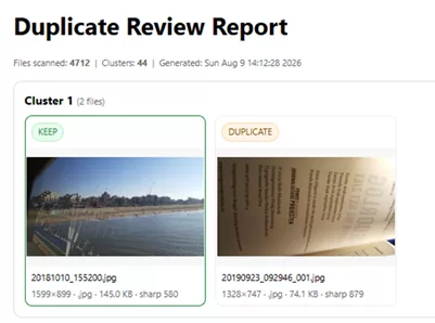
Two visually very different scenes that must have produced more-or-less similar file-metrics. Apparently probing similarities with the commonly used metrics can under specific circumstances produce false positives. With the clustering technique possibly making the consequences even worse.
Before going into the details of clustering, we have to take a closer look at the mathematics used to measure similarity: Hashing and SSIM.
Perceptual Hashing
To detect digital duplicates—both identical and visually similar photos—the principal technique used is called Hashing. A perceptual hashing algorithm creates a short digital fingerprint of multimedia based on what it looks like. Similar files produce (very) close hash values. This differs from cryptographic hashes, which change completely if even one bit is modified. A hash is a short, fixed-length, numerical summary of an image file. This enables fast lookup and indexing. Instead of comparing two full images pixel-by-pixel —which takes time— we can compare their hashes almost instantaneously.
To compare hashes, we compute the Hamming distance. A metric that measures the number of positions where two equal-length strings or binary vectors differ. It counts how many individual symbols or bits must be changed to turn one sequence into the other. String “1011101” and “1001001” differ at the 3rd and 5th positions, giving a Hamming distance of 2.
SSIM Metric
The Structural Similarity Index Measure, or SSIM metric for short, is a method for comparing the quality and similarity of two digital images or videos. Instead of simply counting pixel differences, SSIM, not unlike perceptual hashing, focuses on human perception by measuring luminance, contrast, and structure. Unlike hashing however SSIM does compare images at a pixel-by-pixel level. The score ranges from 0 (no similarity) to 1 (similar).
Pixel-level measures make SSIM metrics inherently slow. The primary use case for SSIM is compression benchmarking, restoration quality checks, and artifact assessment. In duplicate detection, we only sparsely use it for confirmation of borderline cases.
The Culprit: the similarity method
The Python method that does the actual comparison in the previous version of the Dedup-engine is shown in the listing below. It returns True for a pass, False for a failure.
The helper method hamming64() returns the number of different bits between two hash values. In comparing HEIC with JPEG, a little extra tolerance is allowed.
The first test the similarity method applies, is an aspect-ratio comparison between image A and image B. If the difference is greater than 0.02 (the default tolerance), this is considered a failure.
Then the Hamming distance between the hash values of image A and image B is calculated with the helper method. The default threshold here is 8. If the calculated distance is equal to or smaller than this threshold, images with an equal aspect ratio (previous test) are considered to have passed the similarity test.
For borderline cases corroboration from pHash and wHash next to the default dHash is required. Even SSIM can be used for added certainty.
Source Code: Old Matcher
    @staticmethod
    def hamming64(a: int, b: int) -> int:
        return (a ^ b).bit_count()

    def similar(self, A: Features, B: Features) -> bool:
        def _ext(p: str) -> str:
            return os.path.splitext(p)[1].lower()

        def _is_heic_jpeg_pair(a_ext: str, b_ext: str) -> bool:
            heic = {".heic"}
            jpeg = {".jpg", ".jpeg"}
            return (a_ext in heic and b_ext in jpeg) or (b_ext in heic and a_ext in jpeg)

        # aspect ratio guard
        if abs(A.ar - B.ar) > self.cfg.aspect_ratio_tol:
            return False

        d_d = self.hamming64(A.dhash, B.dhash)
        if d_d <= self.cfg.dhash_thr:
            return True

        a_ext = _ext(A.path)
        b_ext = _ext(B.path)
        is_heic_cross = self.cfg.heic_jpeg_relax and _is_heic_jpeg_pair(a_ext, b_ext)
        # Borderline zone where we require corroboration (pHash+wHash).
        # Default: dhash_thr + 2
        borderline_max = self.cfg.dhash_thr + 2
        # HEIC<->JPEG relax: allow a slightly higher dHash only for that crossing, still requiring corroboration.
        if is_heic_cross:
            borderline_max = self.cfg.dhash_thr + max(0, int(self.cfg.heic_jpeg_relax_extra))
        if d_d <= borderline_max:
            d_p = self.hamming64(A.phash, B.phash)
            if d_p <= self.cfg.phash_thr:
                d_w = self.hamming64(A.whash, B.whash)
                if d_w <= self.cfg.whash_thr:
                    # SSIM metric can be calculated using scikit-image or using a CV2 similarity proxy
                    if self.cfg.ssim_check and (_HAS_CV2 or _HAS_SKIMAGE):
                        s = self.quick_ssim(A.path, B.path, self.cfg.ssim_size)
                        return s >= self.cfg.ssim_min
                    return True
return FalseWhy a Strict Threshold can Fail
In practice, this combination of a Hamming distance threshold of 8 combined with an aspect ratio test of 0.02, has been remarkably effective in my photo collections, catching the overwhelming majority of genuine near-duplicates I encountered. Still, we are faced with this, visually obvious, false positive.
One clue is, that, as mentioned above, these images were imported from WhatsApp. A dHash threshold of 8 would in fact be quite strict if the hashes were random 64-bit values, but perceptual hashes are not random. They are highly structured by image content. Thus, our old rule could simultaneously have very high true-positive recall in practice and still produce a nasty false positive.
For genuine near-duplicates, heavy (WhatsApp) compression usually changes pixel values much more than it changes the direction of large-scale brightness transitions in an image. dHash, after aggressive downsampling, basically records the direction of local brightness changes.
So, if the image contains a horizon, a bright sky over a darker foreground, or a document with a broad light-to-dark structure, recompression can destroy detail while preserving many of those directional relationships. That is why dHash is useful. An original photo and its WhatsApp derivative may differ enormously in file size, compression artifacts and fine texture, yet still produce a Hamming distance between 2 – 6 because the underlying coarse luminance geometry survived.
A Strength can be a Weakness
The same property that makes dHash so useful also creates the weakness. Consider what happens through the pipeline: An original smartphone image is resized & recompressed by WhatsApp. This causes loss of fine texture and local detail. Subsequently the Dedup-engine’s dHash computing uses thumbnailing, a reduction to a 9 × 8 grayscale representation, followed by 64 neighbouring brightness comparisons, intentionally discarding a huge amount of semantic information.
For real duplicates, that is beneficial: noise, JPEG blocks and small details disappear, leaving the common structure. But for unrelated images that already have a simple, low-frequency structure, the same process can make them converge. Our example could have come from a textbook. A beach seen through a car window versus the raised page of a document. Semantically they could hardly be more different. Yet both may reduce to something resembling a large bright region plus a broad darker region with strong mostly consistent horizontal gradient.
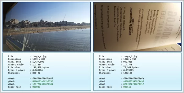
The actual hashes show exactly A: ffffffffffffdfdf and B: fffffffffffffefe. Those hashes are overwhelmingly binary 1s. That tells us that for most of the 64 comparisons, both downsampled images say essentially that their neighbouring horizontal luminance comparisons have the same direction at almost all 64 sampled positions. Only four bits differ. dHash is not saying these images contain the same objects; it says their coarse local brightness-gradient directions happen to be extremely similar.
Compression makes it Worse
Heavy compression tends to remove precisely the information that might otherwise distinguish the two images. Such as fine texture, small edges, subtle tonal variation, local contrast and high-frequency detail.
What survives disproportionately well is broad brightness structure, large boundaries, dominant gradients and overall composition. Those are exactly the things dHash measures.
Thus, we are faced with an interesting paradox. Compression can make dHash more robust for true duplicates while simultaneously making certain unrelated images more collision-prone. The original and its WhatsApp copy become more alike in the feature space that dHash cares about. But in that same reduced feature space an unrelated low-detail image with a similar horizontal gradient can also become more alike.
Aspect-ratio Check
The aspect ratio tolerance at 0.02 is useful, but it is mostly a cheap rejection filter, not strong evidence of identity. For example, image A: 1.77864 and image B: 1.77778, both are essentially 16:9. In a modern photo collection, huge numbers of unrelated images share common (smartphone camera) ratios such as:16:9, 4:3, 3:2 and 1:1.
So, aspect ratio is excellent for saying these definitely cannot be the same image. But relatively weak for saying these probably are the same image. That distinction matters.
Still, the Rule Works Well (most of the time)
The practical observation that the combination of both thresholds together catches almost all true near-duplicates makes sense. Most unrelated photographs are sufficiently structurally different that even after aggressive downsampling their 64 directional comparisons differ substantially. In my testing, genuine near-duplicates frequently produced very small dHash distances, while unrelated photographs were usually much farther apart.
The failures tend to come from a non-random subset of images like the ones discussed here. That is why the problem can remain hidden for a long time. You may get tens of thousands of correct matches before encountering one structurally unfortunate pair when experimenting with images imported from WhatsApp.
Union-Find Makes a Rare False Positive More Expensive
DedupTool uses union-find to turn matching pairs into duplicate clusters. That makes an individual false-positive edge potentially more consequential than it first appears.
Suppose A falsely matches B, while B genuinely matches C and C genuinely matches D:
A — B — C — D. Union-find connects the component. A single incorrect edge can therefore attach an unrelated image—or even another group of images—to an otherwise valid duplicate cluster.
This changes the engineering objective. A matcher that is almost always right at pair level may still not be conservative enough when every accepted pair can influence an entire connected component.
The New Dedup Similarity Evaluation
So, we must take measures and, luckily, the fix is obvious: require corroboration from pHash and wHash for all perceptual matches, not only for the borderline cases. The fix is conceptually straightforward: require corroboration from pHash and wHash for every perceptual match, not only for borderline dHash cases. A dHash distance ≤ 8 is therefore no longer sufficient on its own. The pair must also satisfy the configured pHash and wHash thresholds, with SSIM optionally providing an additional guard during candidate matching.
I wouldn’t frame this core hardening as just more hashes. In the engine the matcher has changed from a single-signal early-accept heuristic into a corroborated evidence policy. dHash can no longer accept a pair by itself. Corroboration is now mandatory, not only for borderline cases. Previously, pHash and wHash were only consulted in the borderline dHash zone above the normal threshold.
The useful property here is not simply that three hashes are better than one. They encode image structure differently. dHash focuses strongly on neighbouring brightness gradients, while pHash represents low-frequency image structure in the frequency domain and wHash derives its representation through wavelet decomposition. Their failure modes therefore do not completely overlap. Requiring them to agree makes it much less likely that one unusually simple gradient structure can determine the result by itself.
Note. Colour hash is also calculated by DedupTool and is useful diagnostic evidence, but it is not currently part of this mandatory acceptance path; the hardening described here specifically concerns corroboration between dHash, pHash and wHash.
Candidate Matching & Cluster Refinement Share One Policy
The new engine version now uses both similar() and similar_to_seed(), that both call the same method evaluate_match() with only the mode changing from “candidate” to “seed“. Thus, the main matcher and cluster refinement now share the hardened policy. The source code is shown in the listing below.
Seed refinement is deliberately stricter, with mode = “seed” a tighter dHash limit is used while still requiring the same pHash and wHash corroboration. This helps reduce transitive bridge effects in union-find clusters.
Source Code: New Matcher
    @staticmethod
    def hamming64(a: int, b: int) -> int:
        return (a ^ b).bit_count()

    def similar_to_seed(self, A: Features, B: Features) -> bool:
        return self.evaluate_match(A, B, mode="seed").accepted

    def similar(self, A: Features, B: Features) -> bool:
        return self.evaluate_match(A, B, mode="candidate").accepted

    def evaluate_match(self, A: Features, B: Features,  *,   mode: Literal["candidate", "seed"] = "candidate", ) -> MatchEvidence:
        if mode not in {"candidate", "seed"}:
            raise ValueError(f"Unsupported match mode: {mode}")
        ar_delta = abs(A.ar - B.ar)
        ar_limit = float(self.cfg.aspect_ratio_tol)
        dh_limit = self._dhash_limit(A, B, mode)
        ph_limit = int(self.cfg.phash_thr)
        wh_limit = int(self.cfg.whash_thr)
        d_d = self.hamming64(A.dhash, B.dhash)
        d_p = self.hamming64(A.phash, B.phash)
        d_w = self.hamming64(A.whash, B.whash)

        common = dict(mode=mode, aspect_ratio_delta=ar_delta, aspect_ratio_limit=ar_limit, dhash_distance=d_d, dhash_limit=dh_limit,
                      phash_distance=d_p, phash_limit=ph_limit, whash_distance=d_w, whash_limit=wh_limit,)
        if ar_delta > ar_limit:
            return MatchEvidence(accepted=False, reason="aspect_ratio", **common)
        if d_d > dh_limit:
            return MatchEvidence(accepted=False, reason="dhash", **common)
        if d_p > ph_limit:
            return MatchEvidence(accepted=False, reason="phash", **common)
        if d_w > wh_limit:
            return MatchEvidence(accepted=False, reason="whash", **common)
        # Cluster refinement intentionally avoids a second expensive SSIM pass using skimage
        if mode == "candidate" and self.cfg.ssim_check and _HAS_SKIMAGE:
            score = self.quick_ssim(A.path, B.path, self.cfg.ssim_size)
            accepted = score >= self.cfg.ssim_min
            return MatchEvidence(
                accepted=accepted,
                ssim_score=score,
                ssim_limit=float(self.cfg.ssim_min),
                reason="accepted" if accepted else "ssim",
                **common,
            )
return MatchEvidence(accepted=True, reason="accepted", **common)SSIM Used Selectively
SSIM can act as an additional guard. On the seed-refinement path, however the engine deliberately avoids another expensive SSIM pass. That is a deliberate performance-safety compromise.
HEIC versus JPEG relaxation is still supported, but no longer weakens corroboration.
The dHash limit may be relaxed for HEIC-JPEG cross-format comparisons, but pHash and wHash must still agree. So, format tolerance no longer means single-hash tolerance.
Explainability
The matcher now returns evidence, not just True or False, Pass or Fail. Match evidence records the following data: aspect-ratio delta & limit, dHash distance & limit, pHash distance & limit, wHash distance & limit, optional SSIM score & limit, the decision: accepted or rejected, and, when failed, the rejection reason. The decisions thus can be documented.
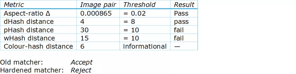
This is a substantial hardening improvement because the system can now explain why a pair was rejected or accepted. For our beach versus document example, the evidence would essentially say: aspect ratio: PASS, dHash: PASS (4 <= 8), pHash: FAIL (30 > 10) and wHash: FAIL (15 > 10), result: REJECT, reason: pHash.
Note. The code is (more or less) fail-fast, so the immediate rejection reason, the first failure, is pHash, while the complete evidence object preserves all three hash distances and limits.
Explicit, Policy-Consistent Evaluation
The implementation calculates the inexpensive hash distances up front and applies the acceptance gates in an explicit sequence: aspect ratio → dHash → pHash → wHash → optional SSIM. Expensive SSIM evaluation is therefore only reached after the cheaper evidence has agreed.
Little Recall Traded for a Much Lower False-Positive Risk
The old matcher was very effective at finding heavily compressed real duplicates because dHash is robust to loss of detail. But that same robustness caused unrelated low-detail compressed images to collapse into similar gradient patterns. The current policy lets dHash propose similarity, but independent perceptual representations must corroborate it before the pair can influence clustering.
The hardened matcher performs more corroboration than before, but repeat scans remain fast because perceptual features are cached in SQLite. On a test library of roughly 4,700 images, the initial scan took 17.1 seconds; a fully cached rerun took 1.7 seconds, and adding two new files still completed in 1.6 seconds because only those files needed re-hashing.
The Final Lesson
A perceptual hash is intentionally lossy. Its usefulness comes from throwing away differences we do not care about. But every discarded distinction also creates the possibility that two unrelated images become indistinguishable in that feature space.
The beach and the document were not similar photographs. They were similar only in one deliberately impoverished representation of those photographs. That distinction is the real bug the old matcher failed to respect. The old engine version treated a sufficiently strong dHash match as proof. The hardened engine treats it as evidence and requires independent corroboration from pHash and wHash before accepting a perceptual duplicate. The same policy is then reused during cluster refinement, with a tighter seed threshold.
Heavy compression does not necessarily break dHash; in many cases it makes dHash excellent at recognizing compressed derivatives. The problem is that compression and subsequent downsampling can strip unrelated images down to the same coarse brightness-gradient pattern as well. The original policy could be very successful overall and still fundamentally unsafe as a single-signal automatic decision rule.
Download Windows Desktop App
For general information on installing and using the Windows application, see this article on the previous version.

A version of the article has also been published on LinkeIn.
Ask a Question or give Feedback about this article